15. Wind Energy Modeling¶

Wind energy analysis is the primary application area for the Nalu-Wind development team. This section describes the theoretical basis of Nalu-Wind from a wind energy perspective, using nomenclature familiar to wind energy experts and mapping it to Nalu-Wind concepts and nomenclature described in previous sections. Hopefully, this will provide an easier transition for users familiar with WRF and SOWFA to Nalu-Wind.

In order to evaluate the energy output and the structural loading on wind turbines, the code must model: 1. the incoming turbulent wind field across the entire wind farm, and 2. the evolution of turbine wakes in turbulent inflow conditions and their interaction with the downstream turbines. First, the governing equations with all the terms necessary to model a wind farm are presented with links to implementation and verification details elsewhere in the theory and/or verification manuals. A brief description of Nalu-Wind’s numerical discretization schemes is presented next. This is followed by a brief discussion of the boundary conditions used to model atmospheric boundary layer (ABL) flows with or without wind turbines (currently modeled as actuator sources within the flow domain).

Currently Nalu-Wind supports two types of wind simulations:

Precursor simulations

Precursor simulations are used in wind applications to generate time histories of turbulent ABL inflow profiles that are used as inlet conditions in subsequent wind farm simulations. The primary purpose of these simulations are to trigger turbulence generation and obtain velocity and temperature profiles that have converged to a statistic equilibrium.

Wind farm simulation with turbines as actuator sources

In this case, the wind turbine blades and tower are modeled as actuator source terms by coupling to the OpenFAST libraries. Velocity fields are sampled at the blade and tower control points within the Nalu-Wind domain and the blade positions and blade/tower loading is provided by OpenFAST to be used as source terms within the momentum equation.

15.1. Governing Equations¶

We begin with a review of the momentum and enthalpy conservation equations within the context of wind farm modeling [CLM+12]. Equation (15.1) shows the Favre-filtered momentum conservation equation (Eq. (2.1)) reproduced here with all the terms required to model a wind farm.

(15.1)¶\[\underbrace{\frac{\partial}{\partial t} \left(\bar{\rho}\, \widetilde{u}_i\right)}_\mathbf{I} + \underbrace{\frac{\partial}{\partial x_j} \left( \bar{\rho}\, \widetilde{u}_i \widetilde{u}_j \right)}_\mathbf{II} = - \underbrace{\frac{\partial p'}{\partial x_j} \delta_{ij}}_\mathbf{III} - \underbrace{\frac{\partial \tau_{ij}}{\partial x_j}}_\mathbf{IV} - \underbrace{2\bar{\rho}\,\epsilon_{ijk}\,\Omega_ju_k}_\mathbf{V} + \underbrace{\left(\bar{\rho} - \rho_\circ \right) g_i}_\mathbf{VI} + \underbrace{S^{u}_{i}}_\mathbf{VII} + \underbrace{f^{T}_i}_\mathbf{VIII}\]

Term \(\mathbf{I}\) represents the time rate of change of momentum (inertia);

Term \(\mathbf{II}\) represents advection;

Term \(\mathbf{III}\) represents the pressure gradient forces (deviation from hydrostatic and horizontal mean gradient);

Term \(\mathbf{IV}\) represents stresses (both viscous and sub-filter scale (SFS)/Reynolds stresses);

Term \(\mathbf{V}\) describes the influence Coriolis forces due to earth’s rotation – see Sec. Section 2.2.1;

Term \(\mathbf{VI}\) describes the effects of buoyancy using the Boussinesq approximation – see Section 2.2.2;

Term \(\mathbf{VII}\) represents the source term used to drive the flow to a horizontal mean velocity at desired height(s) – see Section 2.7; and

Term \(\mathbf{VIII}\) is an optional term representing body forces when modeling turbine with actuator disk or line representations – see Section 15.6.

In wind energy applications, the energy conservation equation is often written in terms of the Favre-filtered potential temperature, \(\theta\), equation, as shown below

(15.2)¶\[\frac{\partial}{\partial t} \left(\bar{\rho}\, \widetilde{\theta}\right) + \frac{\partial}{\partial x_j} \left(\bar{\rho}\, \widetilde{u}_j \widetilde{\theta} \right) = - \frac{\partial}{\partial x_j} \hat{q}_j\]

where, \(\hat{q}_j\) represents the temperature transport due to molecular and SFS turbulence effects. Due to the high Reynolds number associated with ABL flows, the molecular effects are neglected everywhere except near the terrain. Potential temperature is related to absolute temperature by the following equation

\[\theta = T \left ( \frac{\bar{p}}{p_\circ} \right)^{-\left(\frac{R}{c_p}\right)}\]

Under the assumption of ideal gas conditions and constant \(c_p\), the gradients in potential temperature are proportional to the gradients in absolute temperature, i.e.,

\[\left[ \frac{\partial T}{\partial t}, \frac{\partial T}{\partial x}, \frac{\partial T}{\partial y} \right] = \left( \frac{\bar{p}}{p_\circ} \right)^\left(\frac{R}{c_p}\right) \left[ \frac{\partial \theta}{\partial t}, \frac{\partial \theta}{\partial x}, \frac{\partial \theta}{\partial y} \right]\]

Furthermore, ignoring the pressure and viscous work terms in Eq. (2.12) and assuming constant density (incompressible flow), it can be shown that solving the enthalpy equation is equivalent to solving the potential temperature equation. The enthalpy equation solved in wind energy problems is shown below

(15.3)¶\[\frac{\partial}{\partial t} \left(\bar{\rho}\, \widetilde{T}\right) + \frac{\partial}{\partial x_j} \left(\bar{\rho}\, \widetilde{u}_j \widetilde{T} \right) = - \frac{\partial}{\partial x_j} q_j\]

It is noted here that the terms \(\hat{q}_j\) (Eq. (15.2)) and \(q_j\) (Eq. (15.3)) are not equivalent and must be scaled appropriately. User can still provide the appropriate initial and boundary conditions in terms of potential temperature field. Under these assumptions and conditions, the resulting solution can then be interpreted as the variation of potential temperature field in the computational domain.

15.2. Turbulence Modeling¶

LES turbulence closure is provided by the Subgrid-Scale Kinetic Energy One-Equation LES Model or the standard Smagorinsky model for wind farm applications.

15.3. Numerical Discretization & Stabilization¶

Nalu-Wind provides two discretization approaches

Control Volume Finite Element Method (CVFEM)

Nalu-Wind uses a dual mesh approach (see Section 3.1) where the control volumes are constructed around the nodes of the finite elements within the mesh – see Fig. 15.1. The equations are solved at the integration points on the sub-control surfaces and/or the sub-control volumes.

Edge-Based Vertex Centered Scheme

The edge-based scheme is similar to the finite-volume approach used in SOWFA with the nodes at the cell center of the dual mesh.

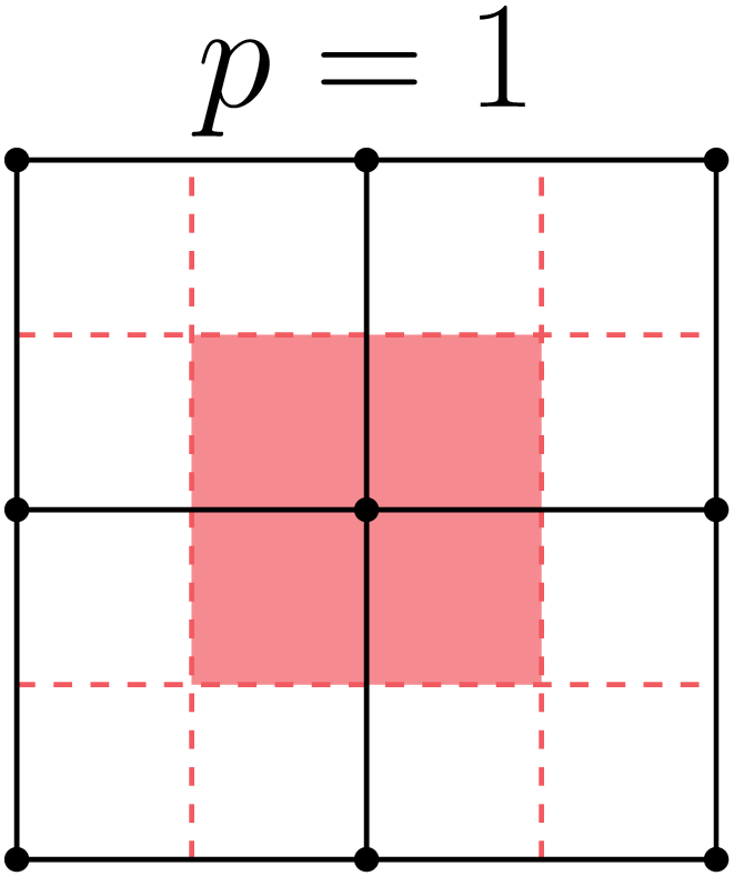
Fig. 15.1 Schematic of HEX-8 mesh showing the finite elements, nodes, and the associated control volume dual mesh.¶

The numerical discretization approach is covered in great detail in Section 3, the advection and pressure stabilization approaches are documented in Section 4 and Section 5 respectively. Users are strongly urged to read those sections to gain a thorough understanding of the discretization scheme and its impact on the simulations.

15.4. Time stepping scheme¶

The time stepping method in Nalu-Wind is described in the Fuego theory manual [Tea16] for the backward Euler time discretization. The implementation details of the BDF2 time stepping scheme used in Nalu-Wind is described here. The Navier-Stokes equations are written as

(15.4)¶\[\begin{split}{\bf F}_i (\rho^{n+1}, u_i^{n+1}, P^{n+1}) - \int \left . \frac{\partial \rho u_i}{\partial t} \right |^{n+1} {\rm d}V &= 0, \\ {\bf F}_i (\rho^{n+1}, u_i^{n+1}, P^{n+1}) - \frac{ (\gamma_1 \rho^{n+1} {u_i}^{n+1} + \gamma_2 \rho^n {u_i}^{n} + \gamma_3 \rho^n {u_i}^{n-1})}{\Delta t} \Delta V &=0,\end{split}\]

where

\[\begin{split}{\bf F}_i (\rho^{n+1} u_i^{n+1}) &= - \int \rho^{n+1} u_i^{n+1} u_j^{n+1} n_j {\rm d}S + \int \tau_{ij}^{n+1} n_j {\rm d}S - \int P^{n+1} n_i {\rm d}S - \int \left(\rho^{n+1} - \rho_{\circ} \right) g_i {\rm d}V, \\ &= - \int u_i^{n+1} \dot{m}^{n+1} + \int \tau_{ij}^{n+1} n_j {\rm d}S - \int P^{n+1} n_i {\rm d}S - \int \left(\rho^{n+1} - \rho_{\circ} \right) g_i {\rm d}V. \\\end{split}\]

and \(\gamma_i\) are factors for BDF2 time discretization scheme (see Section 13). As is typical of incompressible flow solvers, the mass flow rate through the sub-control surfaces is tracked independent of the velocity to maintain conservation of mass. The following conventions are used:

\[\begin{split}\phi^* &= \textrm{ Predicted value of } \phi \textrm{ at } n+1 \textrm{ time step before linear solve} \\ \widehat{\phi} = \phi^{**} &= \textrm{ Predicted value of } \phi \textrm{ at } n+1 \textrm{ time step after linear solve}\end{split}\]

The Newton’s method is used along with a linearization procedure to predict a solution to the Navier-Stokes equations at time step \(n+1\) as

(15.5)¶\[\begin{split}\mathbf{A}_{ij} \; \delta u_{j} &= {\bf F}_i^{*} - \frac{ (\gamma_1 \rho^{*} {u_i}^{*} + \gamma_2 \rho^n {u_i}^{n} + \gamma_3 \rho^n {u_i}^{n-1})}{\Delta t} \Delta V, \\ \textrm{where } \delta u_{j} &= u_i^{**} - u_i^*, \\ \mathbf{A}_{ij} &= \left ( \frac{ \gamma_1 \rho^{*}}{\Delta t} \Delta V \delta_{ij} - \left . \frac{\partial F_i}{\partial u_j} \right |^{*} \right ), \\ \textrm{and } {\bf F}_i^{*} &= - \int u_i^* \dot{m}^* + \int \tau_{ij}^* n_j {\rm d}S - \int P^* n_i {\rm d}S - \int \left(\rho^* - \rho_{\circ} \right) g_i {\rm d}V.\end{split}\]

After each Newton or outer iteration, \(\phi^{**}\) is a better approximation to \(\phi^{n+1}\) compared to \(\phi^*\). \(\rho*\) and \(\dot{m}^*\) are retained constant through each outer iteration. \({\bf F} (\rho^{*} u_i^{**})\) is linear in \(u_i^*\) and hence

(15.6)¶\[{\bf F}_i^* = \left . \frac{\partial F_i}{\partial u_j} \right |^{*} u_j^{*} - \int P^{*} n_i {\rm d}S - \int \left(\rho^{*} - \rho_{\circ} \right) g_i {\rm d}V\]

Applying Eq. (15.6) to Eq. (15.5), we get the linearized momentum predictor equation solved in Nalu-Wind.

(15.7)¶\[\begin{split}{\bf A}_{ij} \; \delta u_j &= \left . \frac{\partial F_i}{\partial u_j} \right |^{*} u_j^{*} - \int P^{*} n_i {\rm d}S - \int \left(\rho^{*} - \rho_{\circ} \right) g_i {\rm d}V \\ & \quad \quad - \frac{ (\gamma_1 \rho^{*} {u_i}^{*} + \gamma_2 \rho^{n} {u_i}^{n} + \gamma_3 \rho^{n-1} {u_i}^{n-1})}{\Delta t} \Delta V \\ {\bf A}_{ij} \; \delta u_j &= \left (\frac{ \gamma_1 \rho^{*}}{\Delta t} \Delta V \delta_{ij} - \left . \frac{\partial F_i}{\partial u_j} \right |^{*} \right ) {u_j}^{*} - \int P^{*} n_i {\rm d}S - \int \left(\rho^{*} - \rho_{\circ} \right) g_i {\rm d}V \\ & \quad - \frac{ (\gamma_2 \rho^{n} {u_i}^{n} + \gamma_3 \rho^{n-1} {u_i}^{n-1})}{\Delta t} \Delta V \\ {\bf A}_{ij} \; \delta u_j & = {\bf A}_{ij} \; u_j^{*} - \int P^{*} n_i {\rm d}S - \int \left(\rho^{*} - \rho_{\circ} \right) g_i {\rm d}V \\ & \quad - \frac{ (\gamma_2 \rho^{n} {u_i}^{n} + \gamma_3 \rho^{n-1} {u_i}^{n-1})}{\Delta t} \Delta V\end{split}\]

\(u_i^{**}\) will not satisfy the continuity equation. A correction step is performed at the end of each outer iteration to make \(u_i^{**}\) satisfy the continuity equation as

\[\begin{split}u_i^{n+1} &= u_i^{**} - \frac{\tau_3}{\rho} {\bf G} \Delta P^{**} \\ \textrm{where } \Delta P^{**} &= P^{**} - P^*\end{split}\]

As described in Section 12.1, the continuity equation to be satisfied along with the splitting and stabilization errors is

(15.8)¶\[{\bf D } \rho u^{**} = b + \left ({\bf L_1} - {\bf D} \tau_3 {\bf G} \right ) \Delta P^{**} + \left ({\bf L_2} - {\bf D} \tau_2 {\bf G} \right ) P^{*}\]

where \(b\) contains any source terms when the velocity field is not divergence free and the other terms are the errors due to pressure stabilization as shown by Domino [Dom06]. The final pressure Poisson equation solved to enforce continuity at each outer iteration is

(15.9)¶\[\begin{split}u^{n+1} &= u^{**} - \frac{\tau_3}{\rho} {\bf G} \Delta P^{**} \\ b + \left ({\bf L_1} - {\bf D} \tau_3 {\bf G} \right ) \Delta P^{**} &+ \left ({\bf L_2} - {\bf D} \tau_2 {\bf G} \right ) P^{*} \\ &= {\bf D}(\rho u^{n+1}) = {\bf D} ( \rho \widehat{u}) - {\bf D }( \tau_3 {\bf G} \Delta P^{**} ) \\ b + {\bf L_1} \Delta P^{**} &= {\bf D} (\rho \widehat{u}) - \left ({\bf L_2} - {\bf D} \tau_2 {\bf G} \right ) P^{*} \\ -{\bf L_1} \Delta P^{**} &= {\bf D} \rho \widehat{u} + {\bf D} \tau_2 {\bf G} P^{*} - {\bf L_2} P^{*} \\ -{\bf L_1} \Delta P^{**} &= - {\bf D} \rho \widehat{u} - {\bf D} \tau_2 {\bf G} P^{*} + {\bf L_2} P^{*} + b\end{split}\]

Thus, the final set of equations solved at each outer iteration is

\[\begin{split}{\bf A}_{ij} \; \delta u_j & = {\bf A}_{ij} \; u_j^{*} - \int P^{*} n_i {\rm d}S - \int \left(\rho^{*} - \rho_{\circ} \right) g_i {\rm d}V \\ & \quad - \frac{ (\gamma_2 \rho^{n} {u_i}^{n} + \gamma_3 \rho^{n-1} {u_i}^{n-1})}{\Delta t} \Delta V \\ -{\bf L_1} \Delta P^{**} &= - {\bf D} \rho \widehat{u} - {\bf D} \tau_2 {\bf G} P^{*} + {\bf L_2} P^{*} + b \\ u_i^{n+1} &= u_i^{**} - \frac{\tau_3}{\rho} {\bf G} \Delta P^{**}\end{split}\]

15.4.1. Approximations for the Schur complement¶

Nalu-Wind implements two options for approximating the Schur complement for the split velocity-pressure solution of the incompressible momentum and continuity equation. The two options are:

\[\begin{split}\tau = \tau_1 = \tau_2 = \tau_3 &= \Delta t \quad \mathrm{Original implementation}\\ & = (A_{ii})^{-1} \quad \mathrm{Alternate algorithm}\end{split}\]

where \(A_{ii}\) is the diagonal entry of the momentum linear system. The latter option is similar to the SIMPLE and PIMPLE implementations in OpenFOAM and is used for simulations with RANS and hybrid RANS-LES models with large Courant numbers.

15.4.2. Underrelaxation for momentum and scalar transport¶

By default, Nalu-Wind applies no underrelaxation during the solution of the Navier-Stokes equations. However, in RANS simulations at large timesteps some underrelaxation might be necessary to restore the diagonal dominance of the transport equations. User has the option to specify underrelaxation through the input files. When underrelaxation is applied, the advection and diffusion contributions to the diagonal term are modifed by dividing these terms by the underrelaxation factor. It must be noted that the underrelaxation is only applied to the advective and viscous contributions in the diagonal term and not the time derivative term.

\[A_{ii} = -\frac{\sum_{i \neq j} A_{ij}}{\omega} + \frac{\gamma_1 \rho \Delta V}{\Delta T}\]

The pressure update can also be underrelaxed by specifying the appropriate relaxation factor in the input file. When this option is activated, the full pressure update, in a given Picard iteration step, is used to project the velocity and mass flow rate and the relaxation is applied to the pressure solution at the end of the Picard iteration.

15.5. Initial & Boundary Conditions¶

This section briefly describes the boundary conditions available in Nalu-Wind for modeling wind farm problems. The terrain and top boundary conditions are described first as they are common to precusor and wind farm simulations.

15.5.1. Initial conditions¶

Nalu-Wind has the ability to initialize the internal flow fields to uniform conditions for all pressure, velocity, temperature, and TKE (\(k\)) in the input file. Nalu-Wind also provides a user function to add perturbations to the velocity field to trigger turbulence generation during precursor simulations. To specify more complex flow field conditions, a temperature profile with a capping inversion for example, users are referred to pre-processing utilities available in NaluWindUtils library.

15.5.2. Terrain (Wall) boundary condition¶

Users are referred to Section 9.3 for the treatment of the terrain BC using roughness models. For enthalpy, users can provide a surface heat flux for modeling stratified flows.

15.5.3. Top boundary condition¶

For problems with minimal streamline curvature near the upper boundary (e.g. nearly flat terrain, negligible turbine blockage), a symmetry BC (slip wall) can be when modeling wind farm problems. By default a zero vertical temperature gradient will be imposed for the enthalpy equation when the symmetry boundary condition is used. If a non-zero normal temperature gradient is required to drive the flow to a desired temperaure profile, e.g., a capping inversion, then the abltop BC can be used. In this case the user_data input normal_temperature_gradient: value will set the normal temperature gradient to value at the top boundary.

For cases with significant terrain features or significant turbine blockage, the abltop BC can also be used to achieve an open boundary that allows for both inflows and outflows at the domain top. See the abltop BC documentation for details.

15.5.4. Inlet conditions¶

Time histories of inflow velocity and temperaure profiles can be provided as inputs (via I/O transfer) to drive the wind farm simulation with the desired flow conditions. See Section 8.3 for more details on this capability. Driving a wind farm simulation using velocity and temperature fields from a mesoscale (WRF) simulation would require an additional pre-processing steps with the wrftonalu utility.

15.5.5. Outlet conditions¶

See the description of open BC for detailed description of the outlet BC implementation. For wind energy problems, it is necessary to activate the global mass correction as a single value of pressure across the boundary layer is not apprpriate in the presence of buoyancy effects. It might also be necessary to fix the reference pressure at an interior node in order to ensure that the Pressure Poisson solver is well conditioned.

15.6. Wind Turbine Modeling¶

Wind turbine rotor and tower aerodynamic effects are modeled using actuator source representations. Compared to resolving the geometry of the turbine, actuator modeling alleviates the need for a complex body-fitted meshes, can relax time step restrictions, and eliminates the need for turbulence modeling at the turbine surfaces. This comes at the expense of a loss of fine-scale detail, for example, the boundary layers of the wind turbine surfaces are not resolved. However, actuator methods well represent wind turbine wakes in the mid to far downstream regions where wake interactions are important.

Actuator methods usually fall within the classes of disks, lines, surface, or some blend between the disk and line (i.e., the swept actuator line). Most commonly, the force over the actuator is computed, and then applied as a body-force source term, \(f_i\) (Term \(\mathbf{VIII}\)), to the Favre-filtered momentum equation (Eq. (15.1)).

The body-force term \(f_i\) is volumetric and is a force per unit volume. The actuator forces, \(F'_i\), are not volumetric. They exist along lines or on surfaces and are force per unit length or area. Therefore, a projection function, \(g\), is used to project the actuator forces into the fluid volume as volumetric forces. A simple and commonly used projection function is a uniform Gaussian as proposed by Sorensen and Shen [SorensenS02],

\[g(\vec{r}) = \frac{1}{\pi^{3/2} \epsilon^3} e^{-\left( \left| \vec{r} \right|/\epsilon \right)^2},\]

where \(\vec{r}\) is the position vector between the fluid point of interest to a particular point on the actuator, and \(\epsilon\) is the width of the Gaussian, that determines how diluted the body force become. As an example, for an actuator line extending from \(l=0\) to \(L\), the body force at point \((x,y,z)\) due to the line is given by

(15.10)¶\[f_i(x,y,z) = \int_0^L g\left(\vec{r}\left(l\right)\right) F'_i\left(l\right) \: \textrm{d} l.\]

Here, the projection function’s position vector is a function of position on the actuator line. The part of the line nearest to the point in the fluid at \((x,y,z)\) has most weight.

The force along an actuator line or over an actuator disk is often computed using blade element theory, where it is convenient to discretize the actuator into a set of elements. For example, with the actuator line, the line is broken into discrete line segments, and the force at the center of each element, \(F_i^k\), is computed. Here, \(k\) is the actuator element index. These actuator points are independent of the fluid mesh. The point forces are then projected onto the fluid mesh using the Gaussian projection function, \(g(\vec{r})\), as described above. This is convenient because the integral given in Equation (15.10) can become the summation

(15.11)¶\[f_i(x,y,z) = \sum_{k=0}^N g(\vec{r}^k) F_i^k.\]

This summation well approximates the integral given in Equation (15.10) so long as the ratio of actuator element size to projection function width \(\epsilon\) does not exceed a certain threshold.

Presently, Nalu-Wind uses an actuator line representation to model the effects of turbine on the flow field; however, the class hierarchy is designed with the potential to add other actuator source terms such as actuator disk, swept actuator line and actuator surface capability in the future. The ActuatorLineFAST class couples Nalu-Wind with NREL’s OpenFAST for actuator line simulations of wind turbines. OpenFAST is a aero-hydro-servo-elastic tool to model wind turbine developed by the National Renewable Energy Laboratory (NREL). The ActuatorLineFAST class allows Nalu-Wind to interface as an inflow module to OpenFAST by supplying the velocity field information.

15.6.1. Nalu-Wind – OpenFAST Coupling Algorithm¶

A nacelle model is implemented using a Gaussian drag body force. The model implements a drag force in a direction opposite to velocity field at the center of the Gaussian. The width of the Gaussian kernel is determined using the reference area and drag coefficient of the nacelle as shown by Martinez-Tossas. [MartinezT17]

\[\epsilon_d = \sqrt{2 \, c_d \, A/ \pi}\]

where \(c_d\) is the drag coefficient, and \(A\) is the reference area. This value of \(\epsilon_d\) ensures that the momentum thickness of the generated wake is of the right size. The velocity sampled at the center of the Gaussian is corrected to obtain the upstream velocity.

\[{\widetilde{u}_i}_\infty = \frac{1}{1 - c_d \, A / (4 \, \pi \, \epsilon_d^2)} {\widetilde{u}_i}_c\]

where \(\widetilde{u_i}_c\) is the velocity at the center of the Gaussian and \({\widetilde{u}_i}_\infty\) is the free-stream velocity used to compute the drag force. The drag body force is then

\[f_d(x,y,z) = \frac{1}{2} \, c_d \, A\, {\widetilde{u}_i}_\infty^2 \, \frac{1}{\pi^{3/2} \epsilon_d^3} e^{-|\vec{r}|^2/\epsilon_d^2}\]

where \(\vec{r}\) is the position vector between the fluid point of interest and the center of the Gaussian force.

The actuator line implementation allows for flexible blades that are not necessarily straight (pre-bend and sweep). The current implementation requires a fixed time step when coupled to OpenFAST, but allows the time step in Nalu-Wind to be an integral multiple of the OpenFAST time step. At present, a simple time lagged FSI model is used to interface Nalu-Wind with the turbine model in OpenFAST:

The velocity at time step at time step \(n\) is sampled at the actuator points and sent to OpenFAST,

OpenFAST advances the turbines up-to the next Nalu-Wind time step \(n+1\),

The body forces at the actuator points are converted to the source terms of the momentum equation to advance Nalu-Wind to the next time step \(n+1\).

This FSI algorithm is expected to be only first order accurate in time. We are currently working on improving the FSI coupling scheme to be second order accurate in time.

15.6.2. Nalu-Wind – Actuator Disk Model via OpenFAST¶

An actuator disk model is implemented in Nalu-Wind by using an OpenFAST actuator line to sample the flow and compute the forcing. The actuator line is held stationary which leads to computational savings during execution because there is only 1 search operation in the initial setup.

The forces are gathered at each actuator line point, and the total force at each discrete radial location (\(r_j\) where \(j \in [1,N_R]\)) is computed using (15.12).

(15.12)¶\[\mathbf{F}_{total}(r_j) = \sum_{i=1}^{N_B} \mathbf{F}(r_j, \theta_i)\]

where \(N_B\) and \(N_R\) are the number of blades and number of radial points respectively.

\(\mathbf{F}_{total}(r_j)\) is then spread evenly across the original actuator line points and additional ‘swept-points’ that are added in between the actuator lines. The swept-points are always uniformly distributed azimuthally, but the number of swept points can either be non-uniformly or uniformly distributed along the radial direction (left and right images in figure Fig. 15.2). The non-uniform distribution uses the distance between points along the embedded actuator line blades as the arc-length between points in the azimuthal direction. This is the default behavior. If uniform spacing is desired then num_swept_pts must be specified in the input deck. This is the number of points between the actuator lines, so in figure Fig. 15.2 the num_swept_pts is 3.

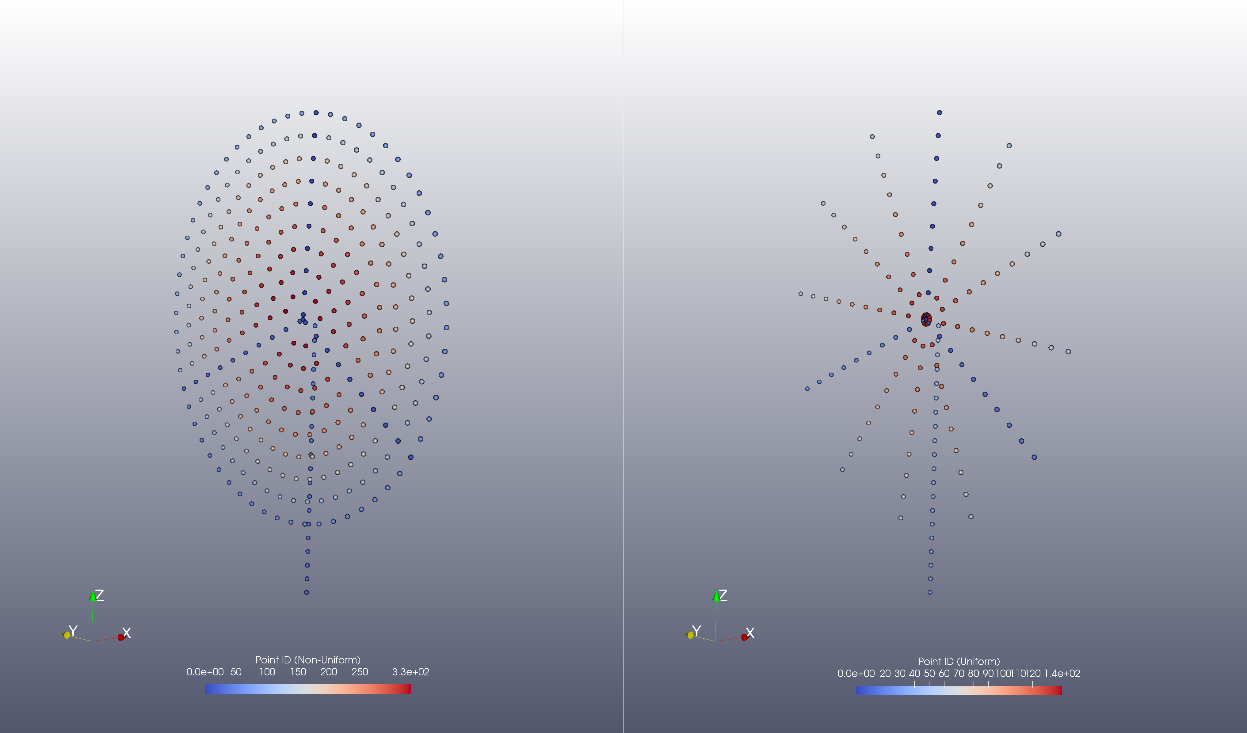
Fig. 15.2 Actuator Disk with non-uniform (left) and uniform (right) sampling in the azimuthal direction.¶

The force that is spread across all the points at a given radius is then calculated as (15.13).

(15.13)¶\[\mathbf{f}(r_j) = \frac{\mathbf{F}_{total}(r_j)}{N_B*(N_{S,j}+1)}\]

where \(N_{S,j}\) is the number of swept points for a given radius. The index j is used because this value varies between radii when non-uniform sampling is applied.