10. Overset

Nalu-Wind supports simulations using an overset mesh methodology to model complex geometries. Currently the codebase supports two approaches to determine overset mesh connectivity:

1. Overset mesh hole-cutting algorithm based on native STK search routines, and

2. Hole-cutting and donor/reception determination using the TIOGA (Topology Independent Overset Grid Assembly) TPL.

The native STK based overset grid assembly (OGA) requires no additional packages, but is limited to simple geometries where the search and hole-cutting procedure works only simple rectangular boundaries (for the inner mesh) that are aligned along the major axes. On the other hand, TIOGA based hole cutting is capable of performing overset grid assembly on arbitrary mesh geometries and orientation, supports generalized mesh motion, and can determine donor/recipient status with multiple meshes overlapping in the same space. A specific use-case for the need to perform OGA on multiple meshes is the simulation of a wind turbine in an atmospheric boundary layer, where the turbine blade, nacelle, and the background ABL mesh might all overlap near the rotor hub.

10.1. Overset Grid Assembly using Native STK Search

The overset descriptions begins with the basic background mesh (block 1) and overset mesh (block 2) depicted in Figure Fig. 10.1. Also shown in this figure is the reduction outer surface of block 2 (light blue). Elements within this reduced overset block will be determined by a parallel search. The collection of elements within this bounding box will be skinned to form a surface on which orphan nodes are placed. Elements within this volume are set in a new internally managed inactive block. These mesh entities are fully removed from the overall matrix for each dof. Elements within this volume are provided a masking integer element varibale of unity to select out of the visualizattion tool. Therefore, orphan nodes live at the external boundary of block 2 and along the reduced surface. The parallel search provides the mapping of orphan node and owning element from which the state can be constructed.

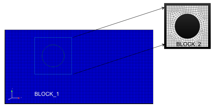
Fig. 10.1 Two-block use case describing background mesh (block 1) and overset mesh (block 2).

After the full search and overset initialization, this simple example yields the original block 1 and 2, the newly created inactive block 3, the original surface of the overset mesh and the new skinned surface (101) of the inactive block (Figure Fig. 10.2).

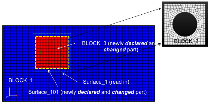
Fig. 10.2 Three-block and two surface, post over set initialization.

A simple heat conduction example is provided in Figure Fig. 10.3 where the circular boundary is set at a temperature of 500 with all external boundaries set to adiabatic.

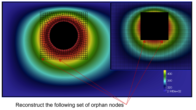
Fig. 10.3 A simple heat conduction example providing the overset mesh and donor orphan nodes.

As noted before, every orphan node lies within an owning element. Sufficient overlap is required to make the system well posed. A fully implicit procedure is provided by writing the orphan node value as a linear constraint of the owning element (Figure Fig. 10.4).

Fig. 10.4 Orphan nodes for background and overset mesh for which a fully implicit constraint equation is written.

For completeness, the constraint equation for any dof \(\phi^o\) is simply,

(10.1)\[\phi^o - \sum N_k \phi_k = 0.\]

As noted, full sensitivities are provided in the linear system by constructing a row entry with the columns of the nodes within the owning element and the orphan node itself.

Finally, a mixed hex/tet mesh configuration example (overset mesh is tet while background is hex) is provided in Figure Fig. 10.5.

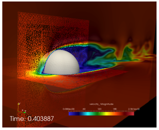
Fig. 10.5 Flow past a three-dimensional sphere using a hybrid topology (hex/tet) mesh configuration.

10.2. Overset Grid Assembly using TIOGA

Topology Independent Overset Grid Assembler (TIOGA) is an open-source connectivity package that was developed as an academic/research counterpart for PUNDIT (the overset grid assembler used in HPCMP CREATE™ A/V program and HELIOS). The base library has been modified to remove the limitation where each MPI rank could only own one mesh block. The code has been extended to handle multiple mesh blocks per MPI rank to support Nalu-Wind’s mesh decomposition strategies.

TIOGA uses a different nomenclature for overset mesh assembly. A brief description is provided here to familiarize users with the differences in nomenclature used in the previous section. When determining overset connectivity, TIOGA ends up assigning IBLANK values to the nodes in a mesh. The IBLANK field is an integer field that determines the status of the node which can be one of three states:

field point

A field point is a node that behaves as a normal mesh point, i.e., the equations are solved on these nodes and the linear system assembly proceeds as normal. The field points are indicated by an IBLANK value of 1.

fringe point

A fringe point is a receptor on the receving mesh where the solution field is mapped from the donor element. A fringe point is indicated by an IBLANK value of -1. Fringe points are how information is transferred between the participating meshes. Note that fringe points are referred to as orphan points in the STK based overset description.

hole point

A hole point is a node on a mesh that occurs inside a solid body being modeled in another mesh. These points have no valid solution for the equations solved and should not participate in the linear system.

In addition to the IBLANK status, the following terms are useful when using TIOGA

donor element

The element that is used to interpolate field data from donor mesh to a recipient mesh. While TIOGA provides flow interpolation routines, the current implementation in Nalu-Wind uses the MasterElement classes in Nalu-Wind to maintain consistency between the STK and the TIOGA overset implementations.

orphan points

The term orphan point is used differently in TIOGA than the STK based overset implementation. TIOGA refers to nodes as orphan points when there it cannot find a suitable donor element for those nodes that are considered fringe points. This can happen when the nodes on the enclosing element are themselves labeled fringe points.

Unlike the STK based hole cutting approach, that uses predefined bounding boxes to determine donor/receptor locations, TIOGA uses the element volume as the metric to determine the field and fringe points. The high level hole cutting algorithm can be described in the following steps:

• Determine and tag hole points that are fully enclosed within solid bodies, tag neighboring points to be fringe points.

• Determine and flag all mandatory fringe points, e.g., embedded boundaries of interior meshes.

• Determine fringe locations for the exterior meshes where information is transferred back from interior meshes to the exterior/background mesh.

In the current integration, only the hole-cutting and donor/receptor information is processed by the TIOGA library. The linear system assembly, specifically the constraint equations for the fringe points are managed by the same classes that are used with the native STK hole-cutting approach.

Figure Fig. 10.6 shows the field and fringe points as determined by TIOGA during the hole-cutting process. The central white region shows the mesh points of the interior mesh. The salmon colored region shows the overlapping field points where the flow equations are solved on both participating meshes. The green-ish boundary shows the mandatory fringe points for the interior mesh along its outer boundary. The interior boundary of the overlap region are the fringe points for the background mesh where information is transferred from the interior mesh. The extent of the overlap region is determined by the number of element layers necessary to ensure adequate separation between the fringe boundaries on the participating meshes.

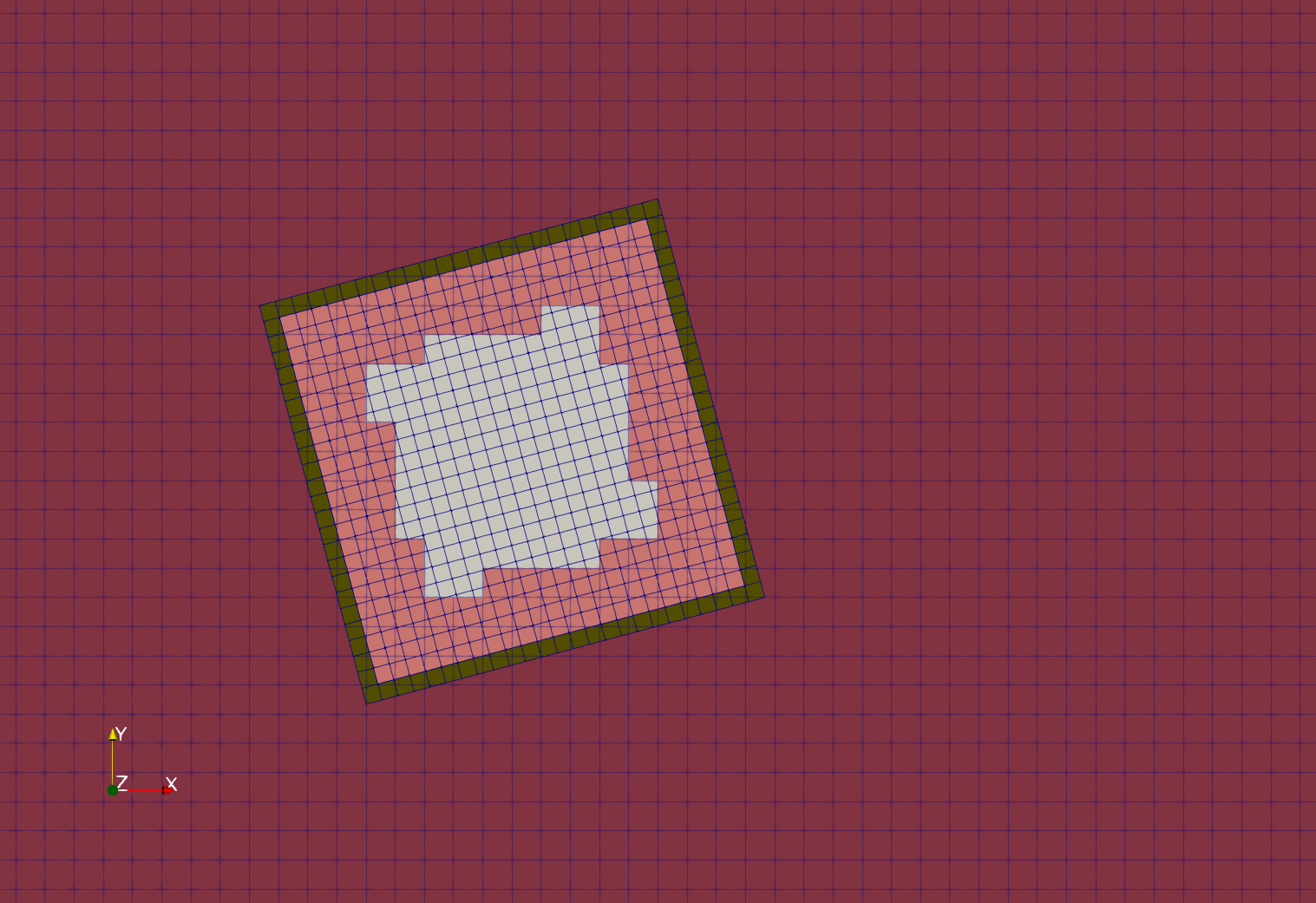
Fig. 10.6 TIOGA overset hole cutting for a rotated internal mesh configuration showing the field and fringe locations.

Figure tioga-overset-cyl shows the resulting overset assembly for cylinder mesh and a background mesh with an intermediate refinement zone. The hole points (inside the cylinder) have been removed from the linear system for both the intermediate and background mesh. The magenta region shows the overlap of field points of the cylinder and the intermediate mesh. And the yellow region shows the overlap between the background and the intermediate mesh.

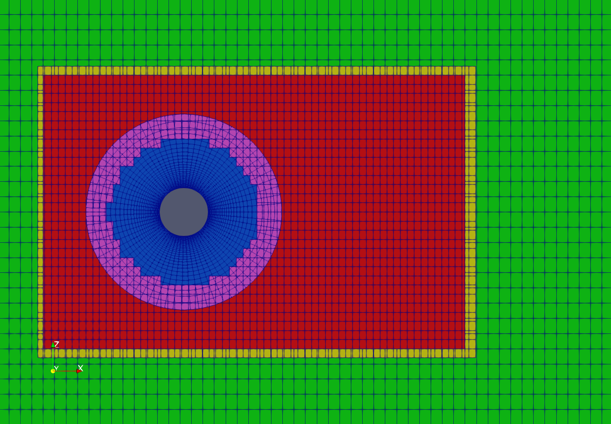
Fig. 10.7 Overset mesh configuration for simulating flow past a cylinder using a three mesh setup: near-body, body-fitted cylinder mesh, intermediate refined mesh, and coarse background mesh.

Figures Fig. 10.8 and Fig. 10.9 shown the velocity and vorticity contours for the flow past a cylinder simulated using the overset mesh methodology with TIOGA overset connectivity.

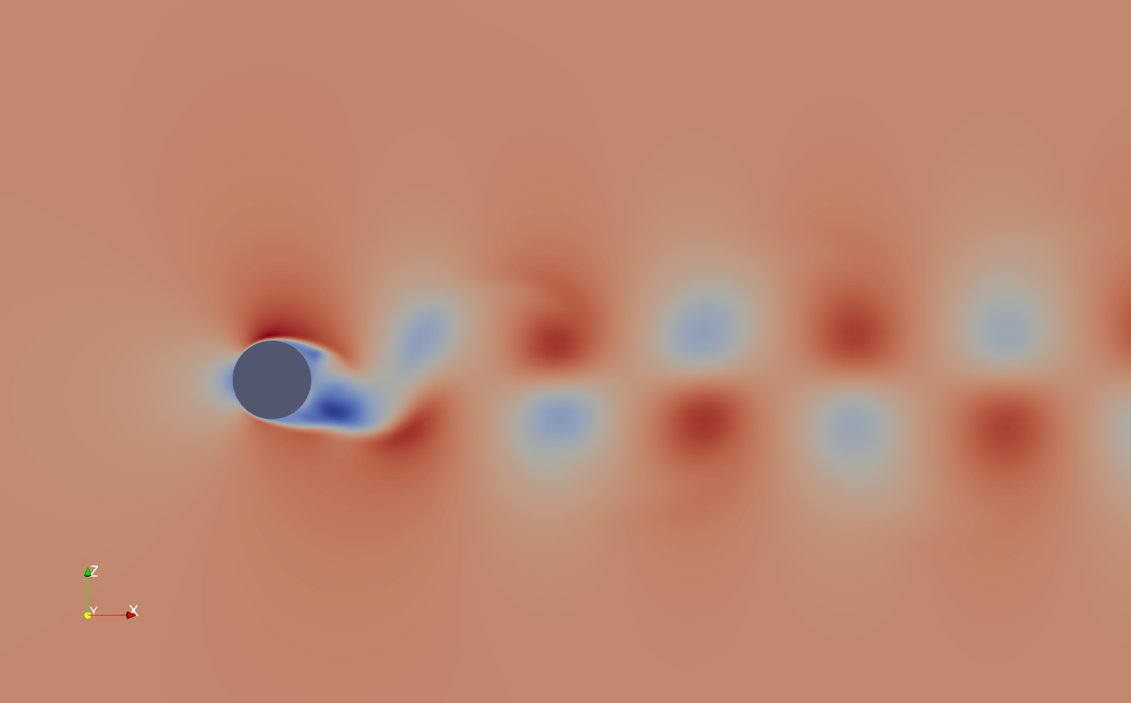
Fig. 10.8 Velocity field for a flow past cylinder simulating using an overset mesh methodology with TIOGA mesh connectivity approach.

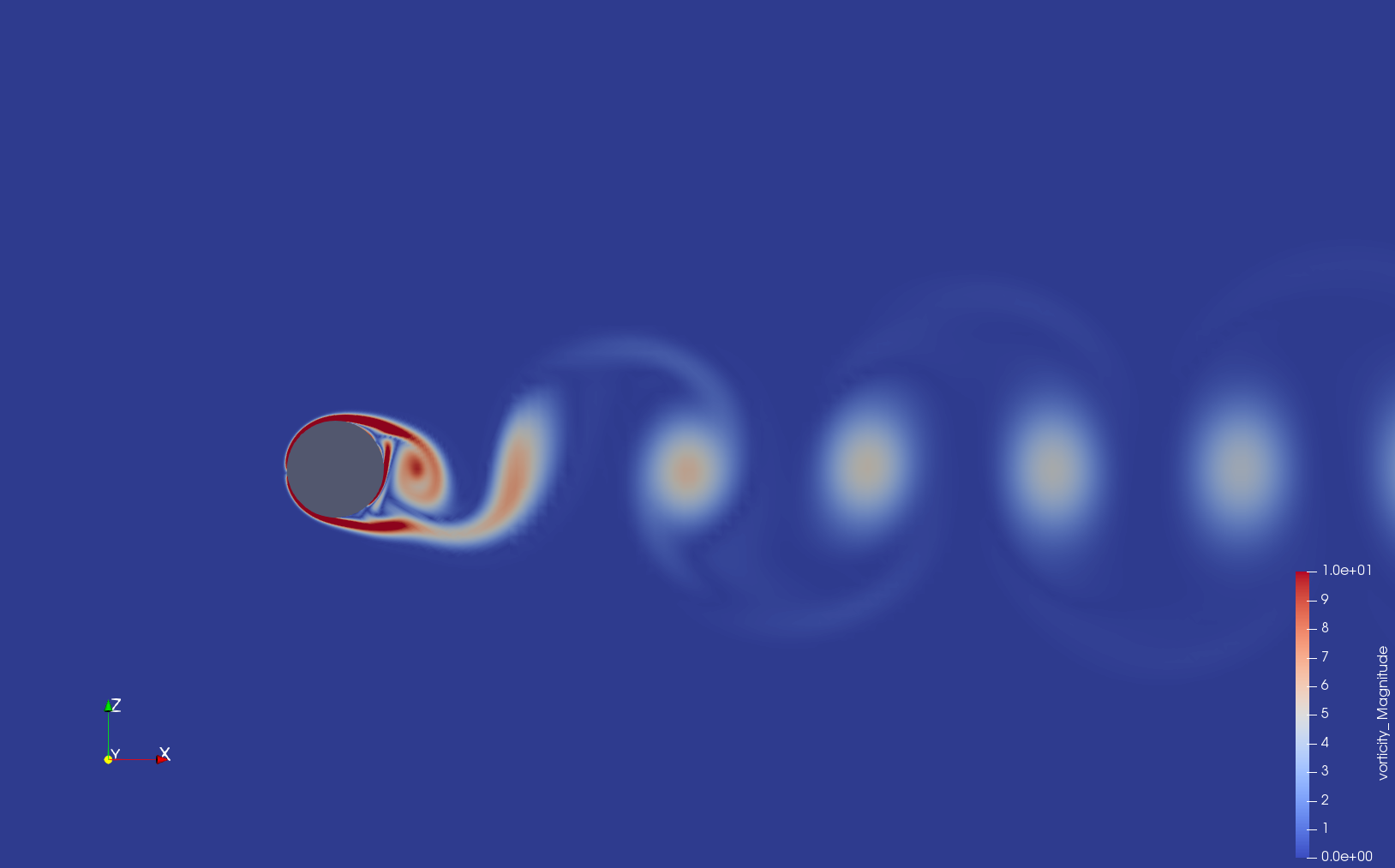
Fig. 10.9 Vorticity field for a flow past cylinder simulating using an overset mesh methodology with TIOGA mesh connectivity approach.